Gradient Harmonized Single-stage Detector

17 Nov 2018

This post introduces the paper ‘Gradient Harmonized Single-stage Detector’, which tries to tackle hard example mining problem. In the end, we compare between GHM and Focal Loss.

This paper tries to handle the long-existing and well-known problems of one-stage detector: the imbalance between the number of positive and negative examples as well as that between easy and hard examples.

For many real-world applications, one-stage detectors seem to be the way compared with two-stage detectors in consideration of efficiency. But meanwhile, one-stage detectors have never reached state-of-the-art performance. There are two well-known problems, which are mentioned as disharmonies and summed up as attribute imbalance in the paper , the huge difference in quantity between positive and negative examples as well as between easy and hard examples.

why does attribute imbalance break detectors

When one attribute of the training set overwhelms another, the model will tend to perform better on this attribute at the cost of bad performance on the other. For example, if there are 1000 negative examples and 10 positive examples in the training set, the model tends to predict everything as negative to get a low loss. It’s the same for easy and hard examples. When there are $10^5$ easy examples and 10 hard examples, hard ones will just be treated as outliers. These hard examples can be a person in Spider-man costume for pedestrian detection or a golden bus for vehicle detection.

related work

Many papers have already tried to handle this issue. One widely used method is Online Hard Example Mining (OHEM). OHEM discards all easy negative examples (easy examples are examples with low losses) and keeps all positive examples no matter whether they are easy or hard. Another famous approach is Focal loss, which adds a factor calculated from losses to the standard cross entropy criterion. It makes easy examples have lower weights and hard examples higher weights. This paper has similar approach as focal loss in the sense of weighing examples differently. While focal loss has focused only on classification criterion, gradient harmonizing mechanism can be applied to both classification and localization criteria without any hyper-parameter. It takes 3 steps to get Gradient Harmonized Mechanism (GHM) loss:

1. calculate gradient norm distribution
2. calculate gradient density
3. calculate GHM loss

gradient norm distribution

The paper argues, that no matter it’s a positive or negative example and no matter how much loss it causes, what really impacts the performance is the imbalanced distribution of gradient norm.

Let $x$ be the output of a model (logits), $p^*$ the ground truth and $L$ the loss function. Gradient norm is defined as:

$$\begin{aligned} g\coloneqq|\dfrac{\partial{L(x, p^*)}}{\partial{x}}| \end{aligned}$$

cross entropy

Consider the binary cross entropy loss:

$$\begin{aligned} L_{CE}(p, p^*)=\begin{cases} -\log(p)&\text{if }p^*=1\\-\log(1-p)&\text{if }p^*=0\end{cases} \end{aligned}$$

where $p=sigmoid(x)$. Then the gradient with regard to $x$:

$$\begin{aligned} \frac{\partial{L_{CE}}}{\partial{x}}&=\begin{cases}1-p&\text{if }p^*=1\\p&\text{if } p^*=0\end{cases}\\&=p-p^* \end{aligned}$$

Then we can get the norm of gradient w.r.t $x$:

$$\begin{aligned} g =|p-p^*|=\begin{cases}1-p&\text{if }p^*=1\\p&\text{if }p^*=0\end{cases} \end{aligned}$$

The value of $g$ implies the example’s impact on the global gradient.

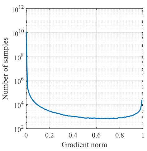
The figure above given by the paper shows the distribution of $g$ from a converged one-stage detection model, where x-axis is gradient norm, and y-axis is number of samples in log scale. From the figure, we can see, that although easy examples have lower individual losses, with extremely large amount, they have probably much bigger impact on the global gradient than hard examples. Moreover, we can see that a converged model still can’t handle some very hard examples whose number is even larger than the examples with medium difficulty. The paper views these as outliers since their gradient directions tends to vary largely from the gradient directions of the large amount of other examples and believes that being forced to learn from these examples might even harm the performance.

smooth $L_1$

Assume we have parameterized offsets, $t=(t_x, t_y, t_w, t_h)$, predicted by box regression and the target offsets, $t^*=(t^*_{x}, t^*_y, t^*_w, t^*_h)$, computed from ground-truth. The smooth $L_1$ loss is calculated as:

$$\begin{aligned} L_{reg}=\sum_{i\in\{x, y, w, h\}}{SL_1(t_i-t^*_i)} \end{aligned}$$

where

$$\begin{aligned} SL_1(d)=\begin{cases}\frac{d^2}{2\delta}&\text{if }|d|<=\delta\\|d|-\frac{\delta}{2}&\text{otherwise}\end{cases} \end{aligned}$$

where $\delta$ is the division point between the quadric part and the linear part.

Since $d=t_i-t^*_i$, the gradient of smooth $L_1$ loss w.r.t $t_i$ can be expressed as:

$$\begin{aligned} \dfrac{\partial{SL_1}}{\partial{t_i}}=\frac{\partial{SL_1}}{\partial{d}}=\begin{cases}\frac{d}{\delta}&\text{if }|d|<=\delta\\sgn(d)&\text{otherwise}\end{cases} \end{aligned}$$

where $sgn$ is the sign function. That means all the examples with $\vert d\vert$ larger than the division point have the same gradient norm $\frac{\partial{SL_1}}{\partial{t_i}}=1$, which makes the distinguishing of examples with different attributes impossible if depending on the gradient norm. Therefore the paper suggested a modified loss function called Authentic Smooth $L_1$( $ASL_1$ ):

$$\begin{aligned} ASL_1(d)=\sqrt{d^2+\mu^2}-\mu \end{aligned}$$

$ASL_1$ shares similar property with $SL_1$ while all the degrees of derivatives are existed and continuous. If we calculate the gradient of $ASL_1$ w.r.t $d$, we can get gradient norm:

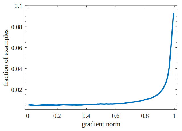
$$\begin{aligned} gr=|\frac{\partial{ASL_1}}{\partial{d}}|=|\frac{d}{\sqrt{d^2+\mu^2}}| \end{aligned}$$

The figure below shows the distribution of gradient norm. It looks different with classification distribution with a large number of outliers. That’s because regression is only preformed on positive examples.

Gradient Density

Gradient density function of training examples is formulated as:

$$\begin{aligned} GD(g)=\frac{1}{l_\epsilon(g)}\sum^N_{k=1}\delta_\epsilon(g_k, g) \end{aligned}$$

where $g_k$ is the gradient norm of the $k$-th example. And

$$\begin{aligned} \delta_{\epsilon}(x,y)=\begin{cases}1&\text{if }y-\dfrac{\epsilon}{2}<=x<y+\dfrac{\epsilon}{2}\\0&\text{otherwise}\end{cases} \end{aligned}$$ $$\begin{aligned} l_\epsilon(g)=\min(g+\frac{\epsilon}{2},1)-\max(g-\frac{\epsilon}{2},0) \end{aligned}$$

The gradient density of $g$ denotes the number of examples lying in the region centered at $g$ with a length of $\epsilon$ and normalized by the valid length of the region.

Gradient Harmonizing Mechanism

With gradient density, we can define the gradient density harmonizing parameter as:

$$\begin{aligned} \beta_i=\frac{N}{GD(g_i)} \end{aligned}$$

where $N$ is the total number of examples. Cos we are going to use it as a normalizer, we can rewrite it as $\beta_i=\frac{1}{GD(g_i)/N}$. The denominator is a normalizer indicating the fraction of examples with neighborhood gradients to the i-th example. If the examples are uniformly distributed with regard to gradient, $GD(g_i)=N$ for any $g_i$ and each example will have the same $\beta_i=1$, which means nothing is changed. Otherwise, the examples with large density will be relatively down-weighted by the normalizer.

After calculating gradient density harmonizing parameter, we can get GHM losses by regarding $\beta_i$ as the loss weight of the i-th example.

We get GHM-C loss by embedding GHM into classification loss:

$$\begin{aligned} L_{GHM-C}&=\frac{1}{N}\sum^N_{i=1}\beta_iL_{CE}(p_i, p^*_i)\\&=\sum^N_{i=1}\frac{L_{CE}(p_i,p^*_i)}{GD(g_i)} \end{aligned}$$

And GHM-R loss by embedding GHM into regression loss:

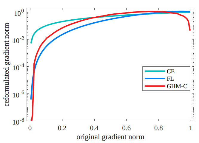
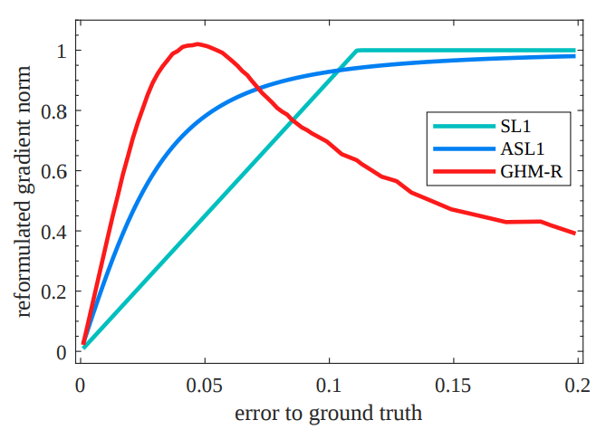
$$\begin{aligned} L_{GHM-R}&=\frac{1}{N}\sum^N_{i=1}\beta_iASL_{1}(d_i)\\&=\sum^N_{i=1}\frac{ASL_{1}(d_i)}{GD(gr_i)} \end{aligned}$$

The figures below are comparison among different classification and regression losses respectively. In classification figure, x-axis is the original gradient norm of CE, i.e. $g=\vert p-p^*\vert$. And y-axis is reformulated gradient norm of different loss functions in log scale. In regression figure, x-axis adopts $\vert d\vert$ for convenient comparison.

Discussion

GHM vs. Focal Loss

GHM and focal loss are almost doing the same thing, since they all weight losses. Although GHM calculates weights in the gradient norm space, they have the same tendency – examples with higher losses contribute higher gradient norm. But GHM focuses on the distribution while focal loss only considers the absolute value of loss.

From the distribution of classification gradient norm, we can see that although small gradient norm tends to have larger quantity, there are still more examples with big gradient norm than the ones with medium norms. That’s the mainly difference between GHM and focal loss in the sense of resulted loss. From the figure which compares focal loss and GHM, we can also easily tell it.

Another difference is that GHM can be applied to regression loss. And compared with traditional $SL_1$ or $ASL_1$ which suggested by this paper, GHM-R lays more emphasis on examples with small gradient norms.