Depthwise Separable Convolution

24 Nov 2018

This post explains a neural network operation called depthwise separable convolution, which trades off between latency and accuracy.

Depthwise separable convolution factorizes a standard convolution into a depthwise convolution and a pointwise convolution. Depthwise convolution captures spatial information of each feature map channel and pointwise convolution combines these information across all channels.

Assume a square input feature and a square output feature. The spatial width and height of the feature map is $D_F$ and the number of input channels is $M$, then we have an input feature map $F$ with size $D_F\times{D_F}\times{M}$ to one network layer. $D_G$ is the spatial width and height of a output feature map and $N$ is the number of output channels. Then the output feature map $G$ has size $D_G\times{D_G}\times{N}$. In a standard convolution assuming square kernel, stride one and padding, the output feature is computed as:

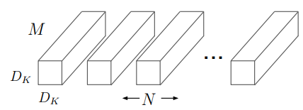
$$\begin{aligned} G_{k,l,n}=\sum_{i,j,m}K_{i,j,m,n}\cdot F_{k+i-1,l+j-1,m} \end{aligned}$$

where $K$ is a convolution kernel with size $D_K\times{D_K}\times{M}\times{N}$, $D_K$ is the spatial dimension of the kernel (as shown in the image below). That means there are $M$ channels of kernels, each of which will do a set of convolution multiplications with each of the $M$ feature map channels. Each convolution multiplication outputs one value. We can imagine it as a kernel sliding over the whole feature map channel and resulting an intermediate output feature channel. Do the same sliding on all $M$ channels separately, we get $M$ intermediate output feature channels. And with the resulted $M$ intermediate output feature channels, we do a pixelwise adding to get one finale output channel with the same spatial size as intermediate output feature channel. Because we have $N$ such kernels, we will get an $N$-channel output feature.

Depthwise separable convolution are made up of two layers: depthwise convolutions and pointwise convolutions. In MobileNets paper, they use both batchnorm and ReLU for both layers. Depthwise convolution applies a single filter per input channel, the same as the first part in standard convolution. The depthwise convolution filters are shown in the figure below.

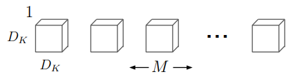
The output of depthwise convolution has the same dimensions as the intermediate output in standard convolution ($D_F\times{D_F}\times{M}$):

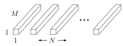
$$\begin{aligned} \hat{G}_{k,l,m}=\sum_{i,j}\hat{K}_{i,j,m}\cdot F_{k+i-1,l+j-1,m} \end{aligned}$$

But in depthwise separable convolution, we don’t have $N$ such kernels, but only one instead. After that, the pointwise convolution is applied to combine the information across channels via $1\times{1}$ convolution. That means there are $N$ $1\times{1}$ convolution kernels, each of which has $M$ channels (as shown in the figure below), so that the final output of the whole depthwise separable convolution block keeps the same as standard convolution.

computational cost

According to the standard convolution equation, we can see that the computational cost is:

$$\begin{aligned} D_K\cdot D_K \cdot M \cdot N \cdot D_F \cdot D_F \end{aligned}$$

For depthwise separable convolution, the computational cost is:

$$\begin{aligned} C_{separable} &= C_{depthwise} + C_{pointwise} \\&=D_K\cdot D_K \cdot M \cdot \cdot D_F \cdot D_F + M\cdot N \cdot D_F \cdot D_F \end{aligned}$$

By expressing convolution as a two step process of filtering and combining we get a reduction in computation of:

$$\begin{aligned} \dfrac{D_K\cdot D_k \cdot M \cdot D_F \cdot D_F + M\cdot N \cdot D_F \cdot D_F}{D_K \cdot D_K \cdot M \cdot N \cdot D_F \cdot D_F} = \dfrac{1}{N} + \dfrac{1}{D_K^2} \end{aligned}$$

With a $3\times 3$ convolution kernel, depthwise separable convolution uses 8 to 9 times less computation than standard convolution.

implementation in Pytorch

After understanding what depthwise separable convolution is doing, it’s trivial to write pytorch code for depthwise separable convolution block:

def conv_dw(input_channel, output_channel, stride):
	return nn.Sequential(
		# assume the kernel size is 3
		# groups=input_channel means each input channel is convolved with its corresponding filter
		# bias=False because batchnorm is applied
		nn.Conv2d(input_channel, output_channel, 3, stride, groups=input_channel, bias=False),
		nn.BatchNorm2d(input_channel),
		nn.ReLU(inplace=True),
		
		nn.Conv2d(input_channel, output_channel, 1, stride=1, bias=False),
		nn.BatchNorm2d(input_channel),
		nn.ReLU(inplace=True),
	)